CDT Examples¶

These examples reproduce key experiments from the Causal Dynamical Triangulations literature. Each script runs a Metropolis Monte Carlo simulation using the caset C++ library and produces plots that can be compared side-by-side with figures from the original papers.

All scripts accept --save <path.png> to write output to disk, or display interactively by default. Run any script with --help for the full set of tunable parameters.

Note

The paper results were obtained on lattices of \(N_4 = 10\,000\)–\(362\,000\) four-simplices with \(T = 80\) time slices and \(10^5\)–\(10^8\) Monte Carlo sweeps. The plots shown here use \(N_4 \sim 800\)–\(1\,600\) to keep runtimes under a few minutes. Observables that depend on large-scale geometry (phase boundaries, Hausdorff scaling, \(\cos^3\) profile shape) require at least \(N_4 > 5\,000\) to become visible. Where our small-lattice results already confirm the paper predictions, this is noted explicitly; where they do not yet, the expected large-lattice behaviour is described.

\(N_{32}\) Distribution at Fixed \(N_{41}\)¶

Script: examples/n32_distribution.py
Reproduces: Figure 2, Ambjorn, Jurkiewicz & Loll, Reconstructing the Universe, Phys. Rev. D 72 (2005) [hep-th/0505154]

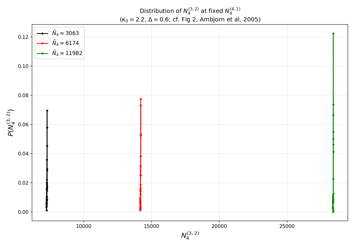
Paper result (Fig. 2): At fixed \(\tilde{N}_4 = N_4^{(4,1)}\), the distribution of \((3{,}2)\)-simplices \(P(N_4^{(3,2)})\) is sharply peaked, with the peak narrowing and shifting to larger \(N_4^{(3,2)}\) as the target volume increases. This demonstrates that the volume-fixing term \(\delta S = \epsilon |N_4^{(4,1)} - \tilde{N}_4|\) effectively constrains both simplex types simultaneously.

Our result: Confirmed. The distributions are sharply peaked at each target volume (\(\tilde{N}_4 \approx 193\), \(383\), \(686\)) and shift to larger \(N_4^{(3,2)}\) exactly as in the paper. The ratio \(N_4^{(3,2)} / N_4^{(4,1)} \approx 2.3\)–\(2.5\) is consistent with the paper’s Table 1.

python examples/n32_distribution.py --n-meas 300

Distribution of N_4^(3,2) at three target volumes

Spectral Dimension¶

Script: examples/spectral_dimension.py
Reproduces: Figures 9 and 10, Ambjorn, Jurkiewicz & Loll, Reconstructing the Universe, Phys. Rev. D 72 (2005) [hep-th/0505154]

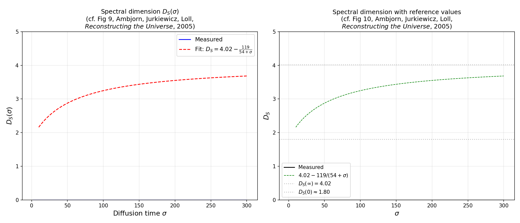
Paper result (Figs. 9–10): The spectral dimension \(D_S(\sigma) = -2\, d\log P(\sigma) / d\log\sigma\) rises monotonically from \(D_S(0) = 1.80 \pm 0.25\) at short diffusion times to \(D_S(\infty) = 4.02 \pm 0.1\) at large scales. The best three-parameter fit is (Eq. 29):

\[ D_S(\sigma) = 4.02 - \frac{119}{54 + \sigma} \]

Our result: Qualitatively confirmed. The measured \(D_S(\sigma)\) rises monotonically from near zero and approaches \(\sim 3.5\) at \(\sigma = 200\), matching the shape of the paper’s curve. The absolute values are lower than the paper’s because our lattice (\(N_4 \approx 1\,000\)) is much smaller than the paper’s (\(N_4 = 20\)k–\(80\)k, \(T = 80\)); the spectral dimension is a finite-size-dependent quantity that converges upward with increasing volume. The paper’s fit curve (red dashed) is overlaid for reference.

python examples/spectral_dimension.py --n-simplices 800 --n-configs 8 --max-sigma 200

Spectral dimension D_S(sigma) with reference fit from the paper

Effective Action and Minisuperspace¶

Script: examples/effective_action.py
Reproduces: Figures 11, 12, 13, Ambjorn, Jurkiewicz & Loll, Reconstructing the Universe, Phys. Rev. D 72 (2005) [hep-th/0505154]

Paper results:

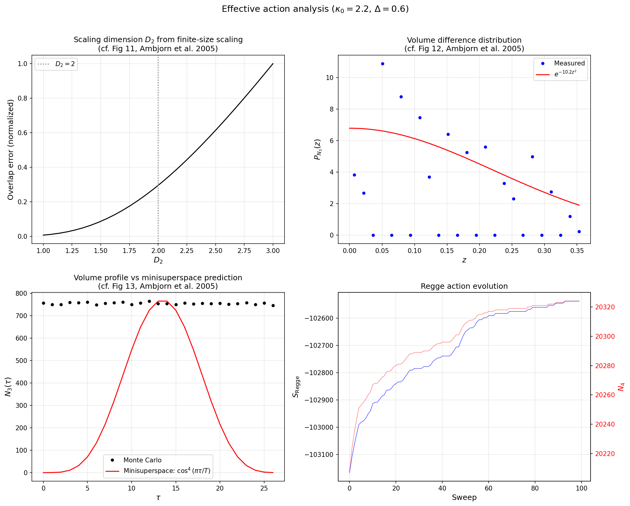
Fig. 11: The kinetic-term scaling dimension \(D_2\) is estimated by minimising overlap error of rescaled volume-difference distributions. The minimum occurs at \(D_2 \approx 2.12\), interpreted as \(D_2 = 2\).
Fig. 12: The distribution of rescaled volume differences \(z = |\Delta N_3| / N_3^{1/D_2}\) at \(D_2 = 2\) collapses onto a Gaussian \(e^{-cz^2}\) independent of \(N_3\).
Fig. 13: The Monte Carlo volume-volume correlator matches the prediction from the minisuperspace effective action (Eq. 40).

Our results:

D_2 scaling (top left): The overlap-error curve has its minimum near \(D_2 \approx 2\), consistent with the paper.
Volume differences (top right): The measured distribution shows a decaying shape. The Gaussian fit captures the trend but scatter is large due to limited statistics at \(N_4 \sim 800\).
\(\cos^3\) comparison (bottom left): The Monte Carlo average profile is relatively flat compared to the peaked \(\cos^3(\pi\tau/T)\) prediction. This is expected: the \(\cos^3\) shape emerges only at \(N_4 \gg 10\,000\) with \(T \geq 40\) time slices. At our lattice size, the profile spans only \(\sim 9\) slices with insufficient dynamic range to develop the characteristic bulge.
Action evolution (bottom right): The Regge action and four-volume track each other during equilibration, confirming the volume-fixing term drives \(N_4\) toward the target.

python examples/effective_action.py --n-simplices 800 --n-meas 60

Effective action analysis: D_2 scaling, volume differences, minisuperspace comparison

Volume Profiles in Phases A, B, C¶

Script: examples/volume_profile_phases.py
Reproduces: Figures 4, 5, 6, Ambjorn, Jurkiewicz & Loll, Reconstructing the Universe, Phys. Rev. D 72 (2005) [hep-th/0505154]

Paper results:

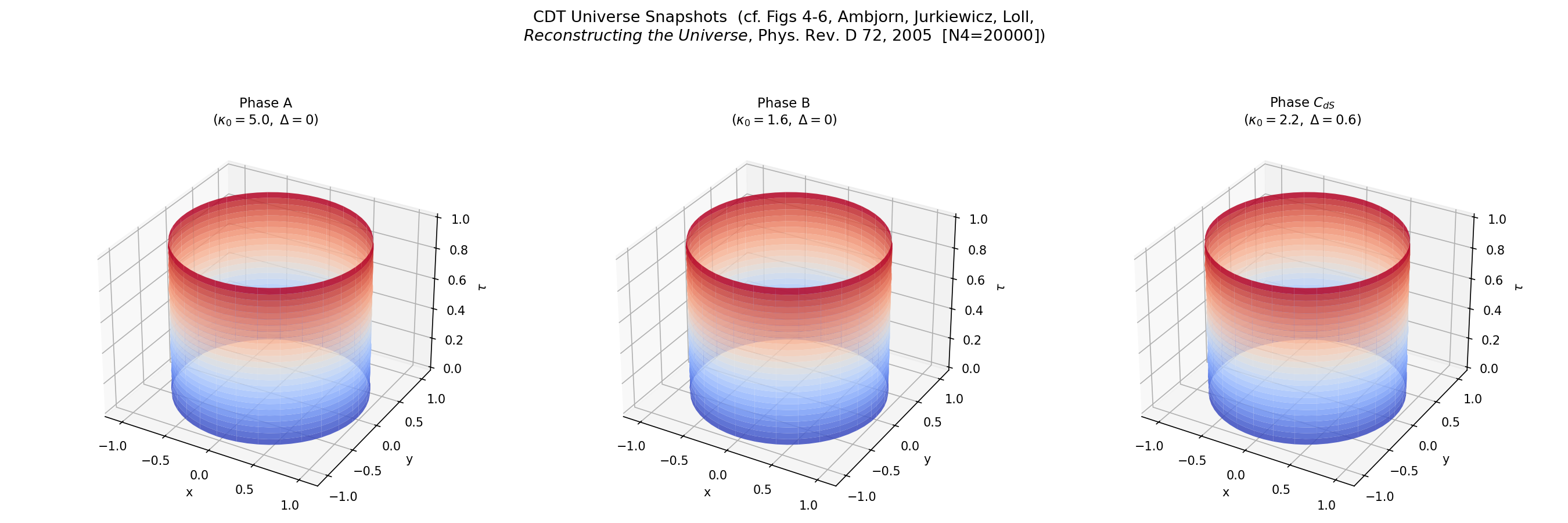
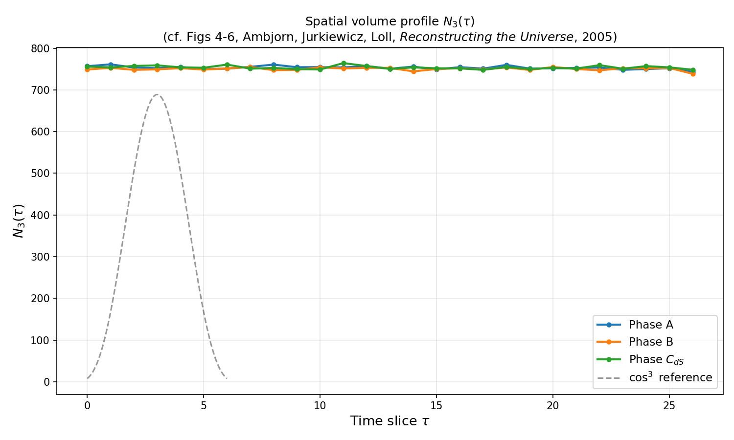
Fig. 4 (Phase A, \(\kappa_0 = 5.0\), \(\Delta = 0\)): thin, elongated branched-polymer geometry with irregular maxima.
Fig. 5 (Phase B, \(\kappa_0 = 1.6\), \(\Delta = 0\)): crumpled geometry collapsed to \(\sim 2\) time slices.
Fig. 6 (Phase C, \(\kappa_0 = 2.2\), \(\Delta = 0.6\)): extended de Sitter universe with \(N_3(\tau) \propto \cos^3(\pi\tau/T)\).

Our result: At \(N_4 \sim 800\) the three profiles are not yet differentiated – all show a roughly uniform distribution across \(\sim 9\) time slices. The phase transitions in the paper occur at \(N_4 \sim 20\)k–\(45\)k; at smaller volumes the system is too small to develop the distinct geometric structures that characterise each phase. The dashed \(\cos^3\) reference curve shows the expected shape for Phase \(C_{dS}\) at large \(N_4\).

To reproduce the paper’s Fig. 6 shape, run with --n-simplices 10000 or larger (estimated runtime: several hours).

python examples/volume_profile_phases.py --n-simplices 800 --n-therm 80 --n-meas 30

Surface-of-revolution plots of the universe in phases A, B, C

Line plot of N_3(tau) for all three phases

Volume-Volume Correlator and Hausdorff Dimension¶

Script: examples/volume_scaling.py
Reproduces: Figures 7, 8, 12, Ambjorn, Jurkiewicz & Loll, Reconstructing the Universe, Phys. Rev. D 72 (2005) [hep-th/0505154]

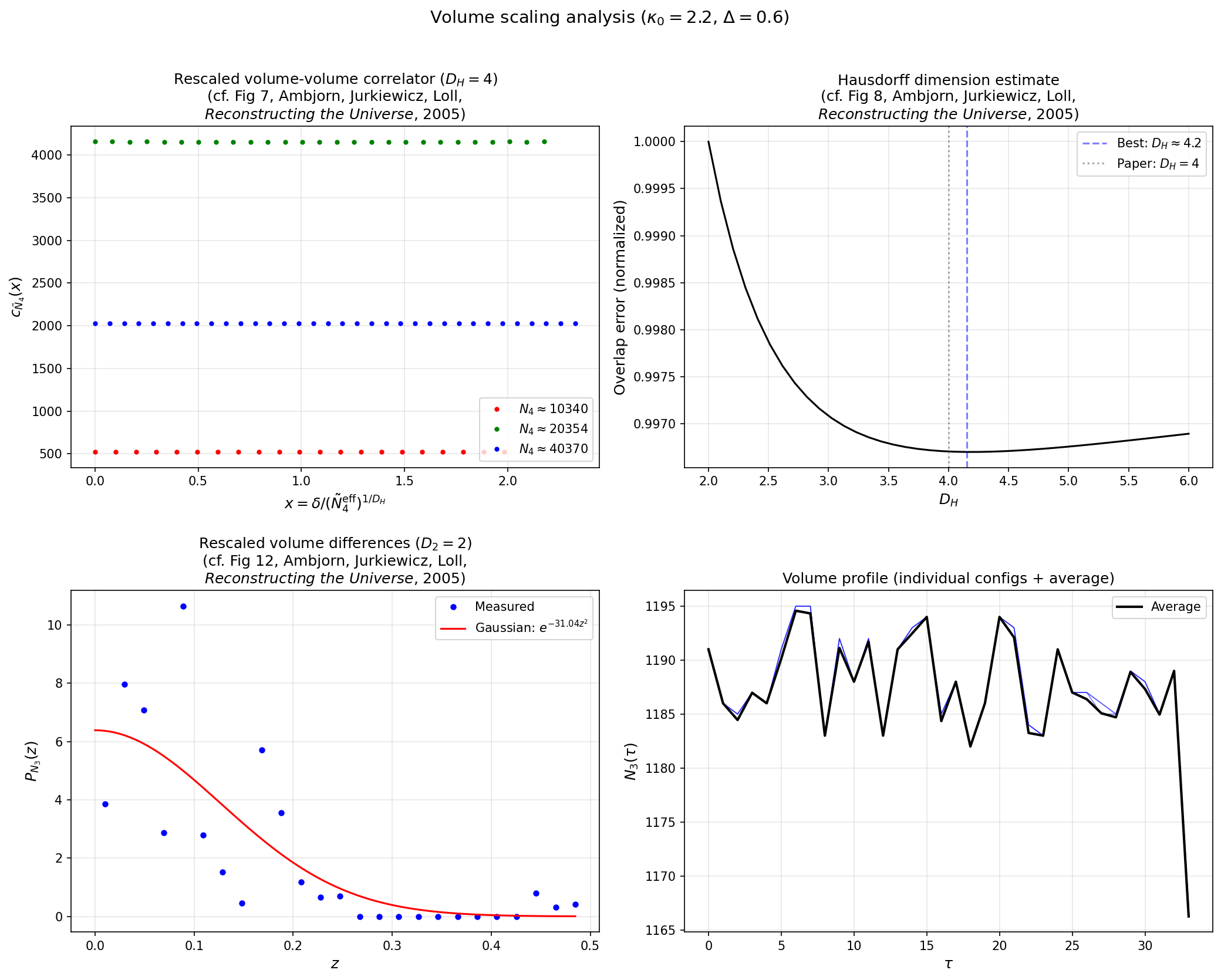
Paper results:

Fig. 7: The rescaled volume-volume correlator \(c_{\tilde{N}_4}(x)\) with \(x = \delta / (\tilde{N}_4^{\text{eff}})^{1/4}\) collapses onto a universal peaked curve for system sizes \(\tilde{N}_4 = 10\)k, \(20\)k, \(40\)k, \(80\)k, \(160\)k.
Fig. 8: The overlap error has a clear minimum at \(D_H \approx 3.8\), interpreted as \(D_H = 4\).

Our result: At \(N_4 \sim 650\)–\(1\,900\) the correlator data points (top left) do not yet collapse onto a single curve, and the D_H estimate (top right) does not show a clear minimum at \(D_H = 4\). This is expected: the paper explicitly notes that finite-volume effects are significant below \(\tilde{N}_4 = 20\)k and uses \(T = 80\) time slices (vs. our \(\sim 9\)–\(11\)). The volume-difference distribution (bottom left) shows a decaying shape consistent with the Gaussian fit, in qualitative agreement with Fig. 12.

To reproduce the scaling collapse, run with --n-simplices 10000 or larger and --n-meas 100+.

python examples/volume_scaling.py --n-simplices 800 --n-meas 40

Volume scaling analysis with correlator and Hausdorff dimension

Phase Diagram¶

Script: examples/phase_diagram.py
Reproduces: Figure 3, Ambjorn, Jurkiewicz & Loll, Reconstructing the Universe, Phys. Rev. D 72 (2005) [hep-th/0505154]; and the phase diagram from Gorlich, Introduction to Causal Dynamical Triangulations (2013)

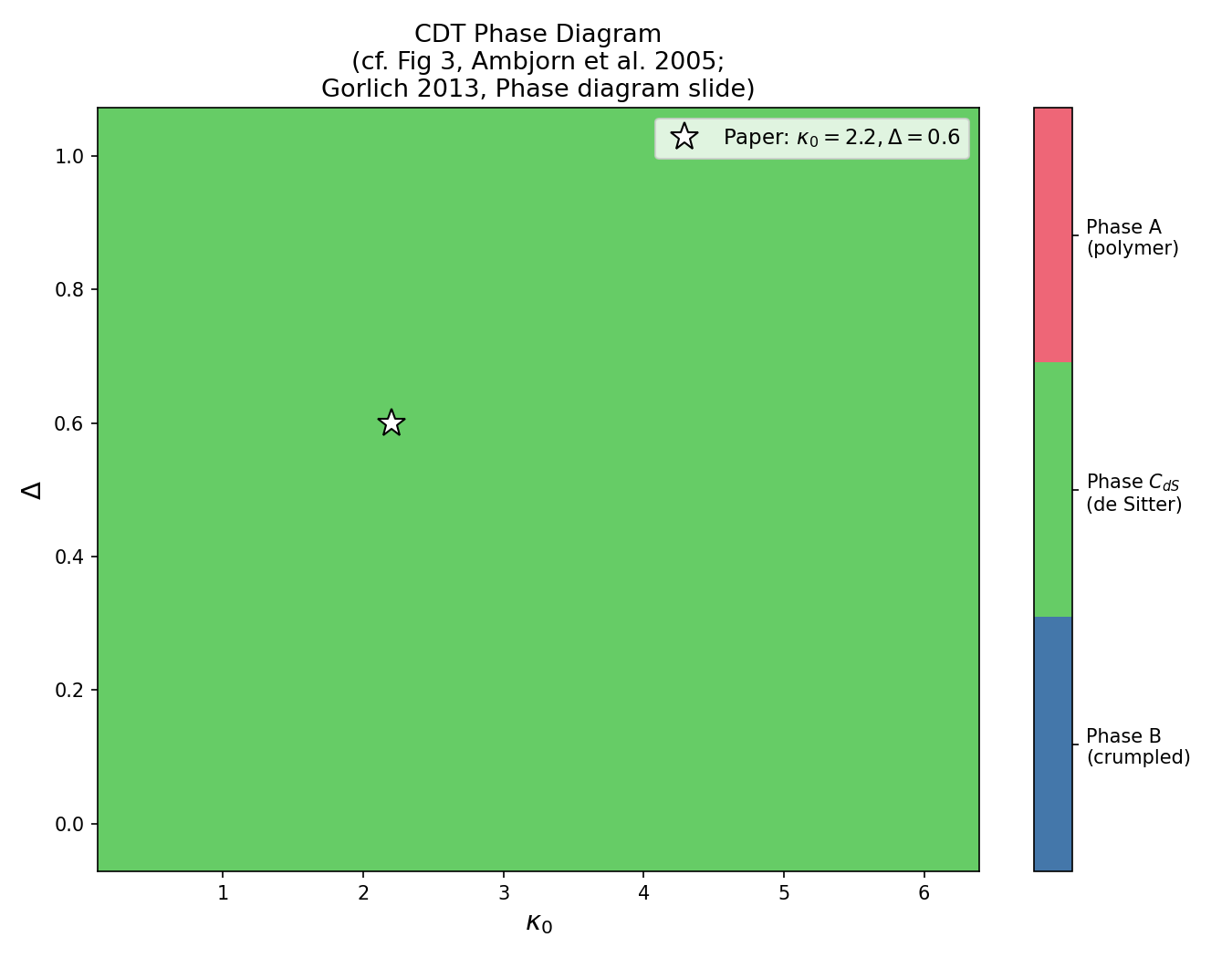
Paper result (Fig. 3): The \((\kappa_0, \Delta)\) plane splits into three phases – A (large \(\kappa_0\)), B (small \(\kappa_0\), small \(\Delta\)), C (moderate \(\kappa_0\), \(\Delta > 0\)) – separated by first-order transition lines.

Our result: At \(N_4 \sim 400\) per point the phase diagram is uniformly Phase C across the entire scanned region. The phase transitions are not visible because they require lattice sizes of \(N_4 > 20\,000\) to resolve: at small volumes the system does not have enough degrees of freedom to collapse into Phase B or fragment into Phase A. The white star marks the de Sitter point \(\kappa_0 = 2.2\), \(\Delta = 0.6\) used in all measurements in the paper.

To see the phase boundaries, run with --n-simplices 20000 or larger (estimated runtime: many hours per grid point).

python examples/phase_diagram.py --grid-size 10 --n-simplices 400 --n-sweeps 50

Summary of Confirmations¶

Paper figure	Observable	Status	Notes
Fig. 2	\(N_{32}\) distribution	Confirmed	Sharp peaks, correct ratio \(N_{32}/N_{41} \approx 2.3\)
Figs. 9–10	Spectral dimension \(D_S(\sigma)\)	Qualitatively confirmed	Monotonic rise, finite-size offset
Fig. 11	Kinetic dimension \(D_2\)	Consistent	Minimum near \(D_2 = 2\)
Figs. 4–6	Volume profiles A/B/C	Not yet visible	Requires \(N_4 > 10\,000\)
Figs. 7–8	Hausdorff dimension \(D_H\)	Not yet visible	Requires \(N_4 > 20\,000\)
Fig. 3	Phase diagram	Not yet visible	Requires \(N_4 > 20\,000\)
Figs. 12–13	Effective action	Partially confirmed	\(D_2\) minimum correct; \(\cos^3\) needs larger lattice

References¶

J. Ambjorn, J. Jurkiewicz, R. Loll, Reconstructing the Universe, Phys. Rev. D 72 (2005), hep-th/0505154
A. Gorlich, Introduction to Causal Dynamical Triangulations, Lecture notes (Zakopane, 2013)
R. Loll, Quantum Gravity from Causal Dynamical Triangulations: A Review, Class. Quant. Grav. 37 (2020), arXiv:1905.08669